Improving the knowledge about carbon cycle processes necessitates a long-term global monitoring strategy.
One critical element in such a strategy is provided by the so-called "top-down atmospheric inversion" method,
which is based on atmospheric concentration measurements from a global network of observation stations. The CO2 concentration in sampled air has the information for source and sink. Therefore the source and sink of CO2 can be calculated from measured CO2 concentration and known transport processes.
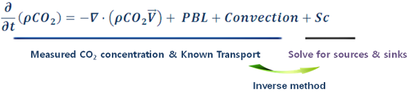
Concept of CarbonTracker. Transfer from observation to information.
First, a prior knowledge of the spatial-temporal distribution of the fluxes to estimate is necessary. Fluxes are provided base components from fossil fuel use, wildfire, vegetation and the oceans. These are ingested into an atmospheric model which simulates the mixing of the air over the whole globe. Simulated concentrations are compared with the observed atmospheric CO2 mole fractions at the location and time when measurements are available. Finally, the inverse modeling of CarbonTracker is to optimize sources and sinks of CO2 to reduce the differences between the simulated CO2 values and the measurements.
Procedures of CarbonTracker. H is a operator representing atmospheric transport. xa and xp are the estimated and a priori flux, respectively.
In particular the following information is exploited in an inverse procedure:
Observations of atmospheric CO2 concentrations: Highly accurate and comparable measurements permit the detection of the atmospheric signatures of the spatial and temporal variations of surface sources and sinks of CO2. The atmospheric observations were obtained from the NOAA ESRL Cooperative Global Air Sampling Network and partner laboratories networks that include flasks, towers, and continuous measurements. Existing atmospheric observing networks focus largely on measurements in the remote marine boundary layer, to avoid contamination by local sources and sinks.
A priori knowledge of sources and sinks: With increasing number of observation data becoming available recently, equally important in increasing the reliability of the atmospheric transport inversion is to increase the reliability of the background CO2 fluxes that are used to derive the a-priori values of CO2 concentration fields for solving the inversion problems. We considered four separate types of CO2 surface fluxes: (1) emissions from fossil fuel use and cement manufacturing, (2) emissions from wildfire , (3) gas exchange with the oceans, and (4) terrestrial biosphere net ecosystem exchange (NEE). The fossil fuel emission distribution was specified from the spatially and temporally-resolved inventories based on the EDGAR database. In addition, the fire module is based on the fPAR-driven Global Fire Emissions Database version 3.1 (GFEDv3.1), which is derived from the CASA biogeochemical model. Over the oceans, a prior information on the sources was specified from the ocean inversion flux based on Takahashi pCO2 estimates. Over the land the a priori source pattern was specified from global carbon fluxes as simulated by the Carnegie-Ames-Stanford Approach (CASA) biogeochemical model. A diurnally varying NEE flux was constructed from two flux components: gross primary production (GPP) and ecosystem respiration (Re).
Transport model to link sources and sinks to atmospheric observations: Surface sources and sinks are prescribed in transport model and converted into atmospheric concentrations after being advected, diffused, and convected. The atmospheric transport is simulated using the global two-way nested Transport Model 5 (TM5) and is forced by the time-varying meteorology from the ECMWF data. The model has 34 levels in the hybrid-sigma coordinate, a global 3° x 2° horizontal resolution with a nested regional grid over Asia at 1° x 1° resolution.
Inversion procedure (Ensemble Data Assimilation): TM5 is used to constrain CO2 fluxes over 11 land and 30 ocean regions. each of the 11 TransCom land regions contains a maximum of 19 ecosystem types. Large regions were used because of the sparseness of the CO2 observation sites. The inverse technique that has been most commonly employed to estimate the carbon flux, requires a prior estimate of the carbon flux in each region to be inverted in order to optimize the impacts of the errors in CO2 observation and in the transport model on the final inverted carbon flux. This optimization procedure is performed by a fixed-lag ensemble Kalman smoother implemented within the atmospheric transport model.